Local governments have made a wide variety of data available at the ZIP code level. A great way of visualizing this information is to use a choropleth map, in which each ZIP code is colored by the intensity of its value for a particular statistic.
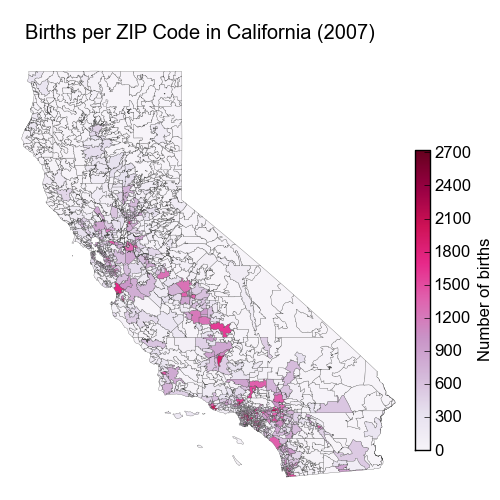
In this article I’ll demonstrate how to produce a ZIP-level choropleth map using freely available tools and data. As an example, we’ll plot the total number of births in 2007 for each ZIP code in California. Here’s an example of the final output:
All the data and script files used in this example are available here. If you would like further information, this page has links to a large selection of ZIP-level data, including population, political and environmental statistics. Also, the website FlowingData has an excellent article on creating maps at the county-level.
OK, let’s get started.
We’ll use Python and matplotlib to create our the map. Make sure you have both installed before proceeding.
The US Census site has lots of great geographic information, including ZIP code boundary files in various formats. We’ll use the ASCII format since it’s easy to read in and manipulate in Python. The 5-digit ZIP code boundary files for each state are available here. This example will use the California file zt06_d00_ascii.zip.
You may already have some data that you wish to plot, but for the purposes of this example we will use birth rate data from the California Department of Public Health. The data in this example was extracted from this Excel file on their site and converted into CSV format (CA_2007_births_by_ZIP.txt is included in here) for processing with Python.
Each ASCII file from the Census website contains boundaries for all the ZIP codes in a state. There are actually two files for each state: a metadata file that ends in ‘a.dat’ and the actual boundary data which ends in just ‘.dat’.
The boundary for each ZIP code has a single main polygon and may also contain several ‘exclusions’ such as islands, lakes, etc. This Python function will read in the data for a given state.
def read_ascii_boundary(filestem):
    '''
    Reads polygon data from an ASCII boundary file.
    Returns a dictionary with polygon IDs for keys. The value for each
    key is another dictionary with three keys:
    'name' - the name of the polygon
    'polygon' - list of (longitude, latitude) pairs defining the main
    polygon boundary
    'exclusions' - list of lists of (lon, lat) pairs for any exclusions in
    the main polygon
    '''
    metadata_file = filestem + 'a.dat'
    data_file = filestem + '.dat'
    # Read metadata
    lines = [line.strip().strip('"') for line in open(metadata_file)]
    polygon_ids = lines[::6]
    polygon_names = lines[2::6]
    polygon_data = {}
    for polygon_id, polygon_name in zip(polygon_ids, polygon_names):
        # Initialize entry with name of polygon.
        # In this case the polygon_name will be the 5-digit ZIP code.
        polygon_data[polygon_id] = {'name': polygon_name}
    del polygon_data['0']
    # Read lon and lat.
    f = open(data_file)
    for line in f:
        fields = line.split()
        if len(fields) == 3:
            # Initialize new polygon
            polygon_id = fields[0]
            polygon_data[polygon_id]['polygon'] = []
            polygon_data[polygon_id]['exclusions'] = []
        elif len(fields) == 1:
            # -99999 denotes the start of a new sub-polygon
            if fields[0] == '-99999':
                polygon_data[polygon_id]['exclusions'].append([])
        else:
            # Add lon/lat pair to main polygon or exclusion
            lon = float(fields[0])
            lat = float(fields[1])
            if polygon_data[polygon_id]['exclusions']:
                polygon_data[polygon_id]['exclusions'][-1].append((lon, lat))
            else:
                polygon_data[polygon_id]['polygon'].append((lon, lat))
return polygon_dataAnd finally here’s the full script that creates the final map:
import csv
from pylab import *

# Read in ZIP code boundaries for California
d = read_ascii_boundary('../data/zip5/zt06_d00')

# Read in data for number of births by ZIP code in California
f = csv.reader(open('../data/CA_2007_births_by_ZIP.txt', 'rb'))
births = {}
# Skip header line
f.next()
# Add data for each ZIP code
for row in f:
    zipcode, totalbirths = row
    births[zipcode] = float(totalbirths)
max_births = max(births.values())

# Create figure and two axes: one to hold the map and one to hold
# the colorbar
figure(figsize=(5, 5), dpi=30)
map_axis = axes([0.0, 0.0, 0.8, 0.9])
cb_axis = axes([0.83, 0.1, 0.03, 0.6])

# Define colormap to color the ZIP codes.
# You can try changing this to cm.Blues or any other colormap
# to get a different effect
cmap = cm.PuRd

# Create the map axis
axes(map_axis)
axis([-125, -114, 32, 42.5])
gca().set_axis_off()

# Loop over the ZIP codes in the boundary file
for polygon_id in d:
    polygon_data = array(d[polygon_id]['polygon'])
    zipcode = d[polygon_id]['name']
    num_births = births[zipcode] if zipcode in births else 0.
    # Define the color for the ZIP code
    fc = cmap(num_births / max_births)
    # Draw the ZIP code
    patch = Polygon(array(polygon_data), facecolor=fc,
        edgecolor=(.3, .3, .3, 1), linewidth=.2)
    gca().add_patch(patch)
title('Births per ZIP Code in California (2007)')

# Draw colorbar
cb = mpl.colorbar.ColorbarBase(cb_axis, cmap=cmap,
    norm = mpl.colors.Normalize(vmin=0, vmax=max_births))
cb.set_label('Number of births')

# Change all fonts to Arial
for o in gcf().findobj(matplotlib.text.Text):
    o.set_fontname('Arial')

# Export figure to bitmap
savefig('../images/ca_births.png')