I recently got engaged to wonderful girl, and as any guy who has gone through this process knows, choosing the right ring can be a tricky decision! Fortunately I had a pretty good idea of my fiance’s tastes: a classic platinum band with a solitaire round cut diamond. Not all diamonds are equal, of course. You may have heard of “the Four C’s” that define the quality of a diamond: cut, clarity, color and carats.
Until I started carefully looking at diamonds (thanks Shane Company) I had no idea what the Four C’s really meant in terms of the physical appearance of a diamond. To my completely untrained eye, carat and color have the greatest impact on the appearance of a diamond but this is a matter of personal preference. What is for certain is that the price of a diamond varies dramatically with the Four C’s. But how exactly does each characteristic affect the price? We can build a statistical model to find out.
The basic steps are:
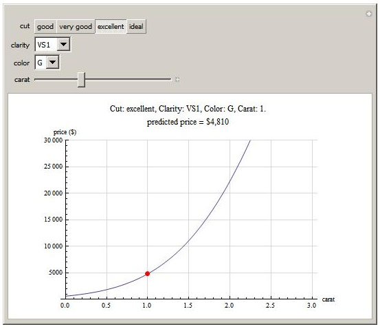
The final result is available at Pricing a Diamond on the Wolfram Demonstrations site. This page gives some detailed background on the steps used to obtain the data and fit the model.
Several websites provide a searchable database of diamonds: Blue Nile and Brilliance.com to name a couple. These sites provide the perfect data source from which to build our statistical model since they have information on cut, carat, color, clarity and price for thousands of diamonds. The trick is getting the information out of the website and into a file for analysis.
All of these sites return their diamond search results in small batches which means it can take a long time to page through manually and save off the HTML for thousands of diamonds. Normally this would be a perfect task for automation using Python’s urllib library. Unfortunately all these sites make extensive use of JavaScript in their search results, and since urrlib doesn’t include a JavaScript engine Python is unable to crawl the search results programmatically.
Instead we will automate the process through Windows Scripting. Using a short VBScript program we can programmatically control Internet Explorer so that it starts paging through the search results and saving off the HTML as if controlled by an invisible hand! It is easiest to do this with the search results from Brilliance.com because the URL from their searches actually contains the page number of the results so it is simple to programmatically construct the URL from a series of integers.
To start, make sure you have Internet Explorer open and pointing to the first page of results from your diamond search on Brilliance.com. Place the following code into a file called get_data.vbs and double-click it in the Windows Explorer. Internet Explorer will start paging through the results, then saving off the HTML files. You may need to tweak some of this code to make it work on your system.
Dim WshShell, objOutputFile, PageCache
Set WshShell = WScript.CreateObject("WScript.Shell")
Set oIE = CreateObject("InternetExplorer.Application")
oIE.Visible = True
oIE.Navigate "http://www.brilliance.com/diamonds/search/Diamond_Results.aspx?SK="

Do While oIE.Busy Or (oIE.READYSTATE <> 4)
    Wscript.Sleep 100
Loop

'Write results to a text file
PageCache = oIE.document.body.innerHTML
Set objFileSystem = CreateObject("Scripting.fileSystemObject")
Set objOutputFile = objFileSystem.CreateTextFile("c:\html\html1.html", 2, TRUE)
objOutputFile.WriteLine(PageCache)
objOutputFile.Close

For i = 2 to 1000

    url = "javascript:SetPageNumber('" & i & "');__doPostBack('lnkCOLOR','');"

    oIE.Navigate url

    Do While oIE.Busy Or (oIE.READYSTATE <> 4)
        Wscript.Sleep 100
    Loop

    'Write results to a text file
    PageCache = oIE.document.body.innerHTML
    Set objFileSystem = CreateObject("Scripting.fileSystemObject")
    fileName = "c:\html\" & i & ".html"
    Set objOutputFile = objFileSystem.CreateTextFile(fileName, 2, TRUE)
    objOutputFile.WriteLine(PageCache)
    objOutputFile.Close

Next
Once you have all the HTML files stored away you can process them using Perl or Python to pull out the data on price, cut, carats, clarity and color. Below is the Python 3.1 code I used to construct a TSV (tab-separated-value) file of the data. The file is available here.
import glob

def process_file(filename):

    pat_tab = re.compile('<TABLE.*?/TABLE>', re.DOTALL)
    pat_tr = re.compile('<TR.*?/TR>', re.DOTALL)
    pat_td = re.compile('<TD.*?/TD>', re.DOTALL)
    pat_entry = re.compile('<TD.*>(.*)</TD>', re.DOTALL)

    f = open(filename, encoding='utf_16')
    text = f.read()
    f.close()
    tab = pat_tab.findall(text)
    tab = [t for t in tab if 'resultGrid' in t]
    if len(tab) != 1:
        return None

    rows = pat_tr.findall(tab[0])

    for row in rows:
        vals = []
        entries = pat_td.findall(row)
        for entry in entries:
            m = pat_entry.search(entry)
            vals.append((m.group(1)))
        if vals[1] == 'Round':
            price = re.sub('[$,]', '', vals[9])
            print(vals[2], vals[3], vals[4], vals[5], price, sep='\t')

print('carat', 'cut', 'color', 'clarity', 'price', sep='\t')
for i in range(1, 1001):
process_file('c:/html/html' + str(i) + '.html')Now that we have the raw data in a nice TSV file, the next step is to build a statistical model that predicts price from the four C’s. The initial step is to recode the data into a purely numerical format. Characteristics such as clarity are rated on a nominal scale from F (flawless) to I3 (heavily included, i.e. flawed). The Diamond Buying Guide has excellent information on the scales for each of the Four C’s. We’ll use Python (again, version 3.1) to translate the nominal characteristics into numeric variables so they can be fit using a generalized linear model.
cut_map = {'Ideal':4,
           'Excellent':3,
           'Very Good':2,
           'Good':1}

color_map = {'D':10,
             'E':9,
             'F':8,
             'G':7,
             'H':6,
             'I':5,
             'J':4,
             'K':3,
             'L':2,
             'M':1}

clarity_map = {'FL':10,
               'IF':9,
               'VVS1':8,
               'VVS2':7,
               'VS1':6,
               'VS2':5,
               'SI1':4,
               'SI2':3,
               'SI3':2,
               'I1':1}

f = open('diamonds.txt')
print(f.readline(), end='')
for line in f:
    (carat, cut, color, clarity, price) = line.strip().split('\t')
    print(carat, cut_map[cut], color_map[color], clarity_map[clarity],
        price, sep='\t')
f.close()
The coded output data is stored in diamonds_coded.txt. Next we’ll use the statistical package R to model the price. Let’s take a quick look at price vs. carats to see what kind of model we should use:
d <- read.delim("diamonds_coded.txt")
x <- tapply(d$price / 1000, round(d$carat), mean)
plot(as.numeric(names(x)), x, type="b", xlab="Carats", ylab="Price ($K)"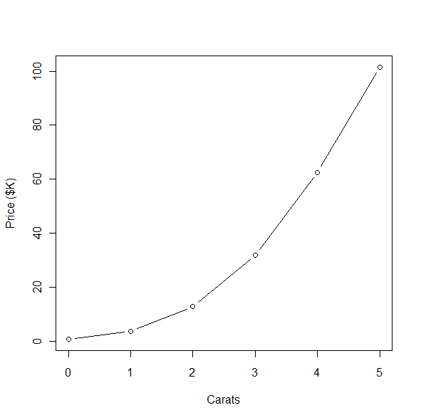
The line shows a clear exponential trend, which suggests using a generalized linear model with a log link to predict price. The code below fits this model, but also includes some higher-order interactions to capture the complex relationships between the four variables and price.
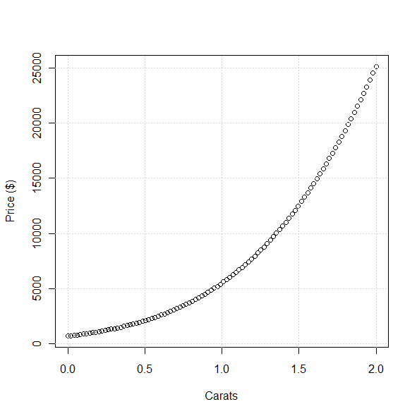
gm <- glm(price ~ cut * clarity * color * carat +
  I(cut^2) + I(clarity^2) + I(color^2) + I(carat^2), family=poisson, d)
testdata <- data.frame(cut=rep(4, 100), clarity=rep(5, 100),
  color=rep(9, 100), carat=seq(0, 2, length=100))
plot(test$carat, predict(gm, test, type="response"), xlab="Carats",
  ylab="Price ($)")
grid()
Here are the predictions from the model for price vs. carats; they closely match the observed data in the previous figure, which is good.
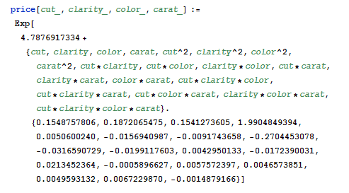
Mathematica 6.0 has the ability to quickly create dynamic user interfaces using the Manipulate function. The last step in this project is to export the model coefficients from R and import them into Mathematica, then wrap a GUI around them using Manipulate so users can interactively explore the relationship between the Four C’s and price. The actual model is fairly complex since it has a lot of interaction terms, but it isn’t too much work to just paste it into a Mathematica notebook and create a function for price. Here is the Mathematica code for the final model:
The final result is available at Pricing a Diamond on the Wolfram Demonstrations site.